How To Create A Vector In R Studio
Vectors
In this chapter we will learn about one of the most basic objects in R, so-called vectors. Before starting, let us do a quick detour to "objects".
Objects in R
R is an object-oriented programming language with the fundamental design principle: Everything in R is an object. In R, objects can be:
- Variables (e.g.,
a,b,result). - Functions (e.g.,
mean(),max(),sin()). - Connection handlers.
- …
Remember the very simple example from the chapter First Steps where we calculated \(a^2\) as follows?
We assign 5 to a. This automatically creates a new object (a) and stores the desired value in it (here 5).
Object orientation: All objects in R have a specific class that can have a set of class-specific attributes as well as methods for certain generic functions. In this simple example, a gets a numeric vector of length 1 (i.e., containing one numeric value).
Know the basics!
Vectors are sometimes also referred to as the 'nuts & bolts' in R as they build the basis for all complex objects such as data frames or fitted regression models. The image below shows a (simplified) schematic overview of how various more complex objects (on the right hand side) are based on vectors (on the left hand side).
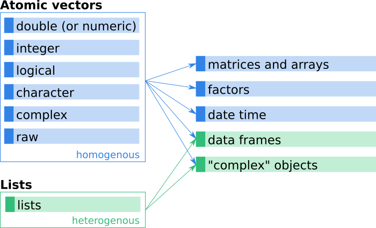
Figure 4.1: Simplified schematic overview of how different R objects, covered in this book, are connected.
Frequently-used data types can also be distinguished by their dimensionality (1-d, 2-d, n-d) and whether they are homogenous (with all elements of the same type) vs. heterogenous (with elements of potentially different types).
| Dimension | Homogenous | Heterogenous |
|---|---|---|
| 1 | Atomic vectors | Lists |
| 2 | Matrix | Data frame |
| \(\ge 1\) | Array |
In this course, we will learn about vectors (atomic vectors), matrices (2-d arrays), factors, date and date time objects, lists, and data frames. In other situations, you will most certainly come across many other more complex objects, but keep in mind that most of them are created by using basic vectors (i.e., lists and atomic vectors).
Thus: Knowing these basics is essential to becoming a good programmer!
Print objects
When working on the interactive R console we can always print objects to see what is stored in them. This can be done by simply entering the name of the object and pressing enter:
## [1] 5 What happens is 'implicit printing' (we have not explicitly asked for it). Explicit printing would be if we call the print() function:
## [1] 5 Both have the same effect when working on the interactive console. When writing scripts, the print() function becomes more important as implicit printing will no longer work (or only in special situations).
One way to (i) create new objects and (ii) directly print them is by adding another pair of round brackets around the command. Instead of doing it in two steps
## [1] 25 we can call (a <- 5^2). The additional brackets cause implicit printing because the result of the assignment to a is evaluated, thus creating the same effect as the two separate lines above.
## [1] 25 This is sometimes useful for brevity, avoiding additional typing and saving some space in the displayed code.
(Atomic) vectors
A vector is nothing else than a sequence of elements of a certain type. R distinguishes vectors with two different modes.
- Atomic vectors: All elements must have the same basic type (e.g., numeric, character, …).
- Lists: Special vector mode. Different elements can have different types.
Lists are deferred to a later chapter and are not important for now. Also, we follow standard albeit somewhat sloppy jargon and refer to atomic vectors simply as vectors while referring to vectors of mode list explicitly as lists (rather than vectors).
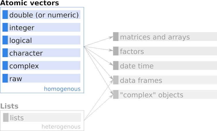
Figure 4.2: Simplified schematic overview of vectors in R which are covered in this chapter.
(Atomic) vectors are the most basic objects in R as they can contain only data of one type (e.g., only numeric values, or only character strings, etc.). Six different types of data can be stored in atomic vectors.
| Type | Example | Comment | |
|---|---|---|---|
| 1 | double (or numeric) | -0.5, 120.9, 5.0 | Floating point numbers with double precision |
| 2 | integer | -1L, 121L, 5L | "Long" integers |
| 3 | logical | TRUE, FALSE | Boolean |
| 4 | character | "R", "5" or 'R', '5' | Text |
| 5 | complex | -5+11i, 3+2i, 0+4i | Real+imaginary numbers |
| 6 | raw | 01, ff | Raw bytes (as hexadecimal) |
Important vector functions
In programming, functions are used to perform a specific task, e.g., manipulate an object, calculate a derived quantity, or investigate existing objects. A few of the most important ones for creating and investigating simple vectors are:
-
c(): Combines multiple elements into one atomic vector. -
length(): Returns the length (number of elements) of an object. -
class(): Returns the class of an object. -
typeof(): Returns the type of an object. There is a small (sometimes important) difference betweentypeof()andclass()as we will see later. -
attributes(): Returns further metadata of arbitrary type.
First example: Let us start with a simple example and assign (<-) the value 1.5 (a numeric floating point number) to an object named x.
We can now use the functions above to investigate this vector and check what the functions return.
## [1] 1 ## [1] "numeric" ## [1] "double" - Length:
1.5is a single numeric value. Thus,xis a vector with only one element and has length1. In R, a single element is always a vector of length 1, there is no special object for single values. - Class: The object is of class "numeric".
- Type: While the class is "numeric" the underlying type is "double". We will come back to what that actually means later.
Second example: We create a new atomic vector with two elements, both integers (as indicated by the L suffix for long integers). c() is the function which combines both values to a new vector, which we (again) store in x. Whatever has been in x previously will be lost, as we overwrite the object.
## [1] 2 ## [1] "integer" ## [1] "integer" - Length: As expected,
length()now returns2as we have stored two elements. - Class and type: Both functions return
"integer".
Third example: As a last example let us create a character vector. A character (or character string) is nothing else but "text", declared in R either by double quote "..." or single quotes '...'. In this case we store two character strings with short text snippets in a new vector called y:
## [1] 2 ## [1] "character" ## [1] "character" - Length: The length is 2 as our atomic vector
ycontains two character strings ("this is"and"just some text"). Note thatlength()does not count the number of individual characters, but the number of elements in our vectory. Feel free to trynchar(y)and note the difference. - Class and type: Twice the same, class and type are identical.
Double (or numeric)
One atomic data class is the double class (double precision floating point values). Double is actually not often used in R, objects of type double are simply called numeric and the class of floating point numbers will be "numeric".
## [1] 1.5 Note: the number 10 will also be numeric (double) as 10 is interpreted as 10.000.
## [1] 10 ## [1] "numeric" Integers
A second atomic class is the integer class. Integers can explicitly be defined using the L ("Long") suffix. While 10 will be double (or numeric; 10.0), 10L defines an integer (natural number).
## [1] 10 ## [1] "integer" This is not important most of the time when you are using R. Except when it is! There are some situations where integers are required!
Logical
Logicals are rather simple as they can only take up two different values: either TRUE or FALSE.
## [1] TRUE ## [1] FALSE ## [1] "logical" Note: TRUE and FALSE must be written without quotation marks (they are logicals not characters).
Characters
The last atomic class we will deal with is the character class. A character is basically just a text and can be of any length.
## [1] "Austria" ## [1] "Max Konstantin Mustermann (AT)" ## [1] "character" Checking class/type
As shown, class() and typeof() can be used to determine the class and type of an object. Both functions return a character vector which contains the name of the class/type (e.g., "numeric" or "integer").
Alternatively, a range of functions exist to check whether or not an object is of a specific type. These very handy functions return either a logical TRUE if the input is of this specific type, or FALSE if not. Examples are:
-
is.double() -
is.numeric() -
is.integer() -
is.logical() -
is.character() -
is.vector() - … and many more.
Some examples:
## [1] FALSE ## [1] TRUE ## [1] TRUE ## [1] TRUE These functions return to us one single logical value TRUE if the object is of a specific class/type, and a FALSE if not.
Double vs. numeric
Let's make things a bit more complicated. If you are new to programming this might be a bit confusing. However, at some point it will get important to know that there is a small but important difference between "numeric" and "double".
For those who already have a background in programming I would like to clarify the language. If you are coming from another programming language you might be familiar with objects of type "double", "real", "float", and "integer". A "double" is a double precision floating point numeric value (e.g., 0.001234). Depending on the programming language they might be referred to as "double", "real", or "float" which are basically the same. An "integer" is also a numeric value but from \(\pm \mathcal{N}_0\) ([..., -3, -2, -1, 0, 1, 2, 3, ...]; positive and negative natural numbers including zero). As we have learned, R is based on C and, thus, shares the data types "double" and "integer" with C. However, there is a difference between the class of an object in R and the type (which is the underlying type).
Let us check what class() and typeof() returns for 1, 1.0, and 1L:
| x | class(x) | typeof(x) | is.double(x) | is.integer(x) | is.numeric(x) |
|---|---|---|---|---|---|
1 | numeric | double | TRUE | FALSE | TRUE |
1.0 | numeric | double | TRUE | FALSE | TRUE |
1L | integer | integer | FALSE | TRUE | TRUE |
The table shows (left to right) the value which is checked (x), the R class of the object x, the type of x, and three checks: whether the value x is double, numeric, or integer (is.*()).
-
1and1.0: are of class "numeric". The underlying data type in C is "double", thus bothis.double()andis.numeric()returnTRUE. -
1L: this is how an integer is specified in R.1Lis of class "integer" and the underlying C type is also "integer", however, an integer in R is also threated as "numeric"! Thusis.numeric()returnsTRUEas well.
Why? Well, the philosophy is that one can use both for mathematical operations. In R there is no difference between 5L^2L, 5L^2.0, and 5.0^2L as in some other programming languages. Thus, is.numeric() basically tells us whether or not we can use this specific object (x) for mathematical calculations.
Keep this in mind, we may get back to it here and there, but we will not use the small but sometimes important difference between "double" and "numeric" often.
Missing values
One additional important element is the missing values. R knows two types of missing values: NaN and NA. NaN is "not a number" and results from mathematical operations which are illegal/invalid. NA on the other hand stands for 'not available' and indicates a missing value. NAs can occur in all the vectors discussed above, and keep their class.
-
NaN: Mathematically not defined (and always of classnumeric). -
NA: Missing value,NA's still have classes! -
NaNis alsoNAbut not vice versa.
Example for NaN : Zero devided by zero (0 / 0) is not a valid mathematical operation, wherefore the result of the devision is NaN.
## [1] NaN Let us check the class and see if the object x is 'not a valid number' (is.nan()) and/or a missing value (is.na()).
## [1] TRUE ## [1] TRUE Note: Missing values in R still have a class. We can have missing numeric, integer, logical, or character missing values. They all look the same, but have a class attached to it.
## [1] "numeric" When defining a new object and storing a single missing value on it (with x <- NA), it will be 'logical' by default. We can, however, convert them (if needed).
## [1] NA ## [1] "logical" ## [1] NA ## [1] "integer" ## [1] NA ## [1] "character" As show, all three objects (x, y, z) look identical and contain one missing value. However, the class of the three objects differs. More about missing values in the corresponding sections where they are getting important.
Creating vectors
Concatenating values c()
As quickly shown earlier, c() can be used to combine (one or) multiple elements to a new vector. An example:
## [1] 1.5 1000.0 0.1 This creates a numeric vector of length 3 with the three elements 1.5, 1000, and 0.1 (in this order).
Important: As mentioned at the very beginning of this chapter, vectors can only contain data of one type! We cannot easily mix e.g., a character string with numeric values or vice versa. It is possible, but we need to take care of what happens in this case. We will come back to that later (subsection Coercion (mixing objects)).
In the same way we can create vectors of other types, e.g., a character vector with three elements:
## [1] "Austria" "Tyrol" "Innsbruck" As each element (e.g., "Austria") itself can be seen as a character vector of length one, c() can also be seen (and used) to combine vectors just the same way as used for elements.
## [1] "Austria" "Tyrol" "Innsbruck" "Germany" "Berlin" "Berlin" ## [1] 6 We could, of course, repeat this example for all atomic vectors including doubles (numeric), logical, character, integer, and complex values (try it yourself!):
x <- c(0.5, 0.6, 0.7) # double x <- c(TRUE, FALSE, TRUE) # logical x <- c(T, F, T) # logical (!!!) x <- c("a", "b", "c") # character x <- c(1L, 2L, 3L, 4L) # integer x <- 15 : 20 # integer x <- c(1 +0i, 2 +4i, 5 +2i) # complex Warning: The example above shows that you could also use T and F as an abbreviation for TRUE and FALSE which you may see frequently when you 'google' something. Please don't do that! T and F are not protected and can be changed. Below we re-define or overwrite T with "bar" and F with "FOO". Thus, c(T, T, F, T) becomes something completely different. Even worse: Imagine what happens if I re-define T <- FALSE and F <- TRUE.
## [1] TRUE TRUE FALSE TRUE ## [1] "foo" "foo" "bar" "foo" Thus, get used to TRUE and FALSE from the beginning. T and F is shorter, but you might run into strange problems at some point which can be avoided by just not using these abbreviations.
Function vector()
An alternative way to create a vector of a specific type and length is the function vector(). vector() requires two input arguments, namely the type of the vector (or 'mode') and the length of the vector.
## [1] 0 0 0 0 0 ## [1] "" "" "" As you can see both vectors are empty. The default value of numeric vectors is 0, the default for character vectors is "" (just an empty character string, a text without any characters in it), and FALSE for logical vectors.
Numeric sequences
Regular sequences can be created using the function seq() and its shortcuts seq.int(), seq_along(), and seq_len().
- Sequences: sequences are a set of numeric or integer values between two well defined points (
fromandto) with an equidistant spacing. By default the spacing/increment is1Lbut can be explicitly specified using thebyargument. - Repeat: Repeat allows to repeat a number (or a set of numbers) in different ways. We can repeat one element several times, repeat a vector multiple times, or repeat the elements of a vector multiple times.
Numeric sequences: We can create numeric sequences using the seq() (generic function) or seq.int() (internal/primitive function). You can try it out yourself, seq() and seq.int() would do the very same in the examples below. Some times it can be beneficial to use seq.int() as it might be much faster, but a bit less flexible. To create a sequence, we have to at least specify three input arguments:
-
from: Where to start the sequence. -
to: Where to end the sequence. -
lengthorby: either define the length of the resulting vector, or the increment by which the values change. Note: iftois less thanfrom,bymust be negative (decreasing sequence). Else you'll get an error.
## [1] 1.50 1.75 2.00 2.25 2.50 ## [1] 4.0 3.5 3.0 2.5 2.0 1.5 1.0 0.5 0.0 -0.5 -1.0 -1.5 -2.0 -2.5 -3.0 ## [16] -3.5 -4.0 Technically, seq() can also be used to create integer sequences. However, this only works if all three arguments from, to, and by (default is 1L) are given, and all are integers!
## [1] 10 20 30 40 50 60 70 80 90 100 ## [1] "integer" ## [1] 10 20 30 40 50 60 70 80 90 100 ## [1] "numeric" Thus, in practice, you should never rely on the class of the sequence returned by seq().
Integer sequences: There are three distinct functions to create proper integer sequences.
-
<from>:<to>: Two values separated by a colon (:); creates sequences in steps of+1or-1. If<from>is an integer (or a numeric value without decimals), an integer sequence will be created. -
seq_along(x): Creates a sequence from1Ltolength(x)wherexis an existing object (e.g., a vector). -
seq_len(n): creates a sequence between1Landn.
Two examples for <from>:<to>:
## [1] 1 2 3 4 ## [1] "integer" ## [1] 30 29 28 27 26 25 ## [1] "integer" To be able to use seq_along() we need an object along which we would like to create the integer sequence. Let us assume we have a character vector cities (see below), seq_along() will return a sequence counting from 1 up to the number of elements in names.
## [1] 1 2 3 4 5 Last but not least, seq_len() simply creates an integer sequence from 1L to n:
## [1] 1 2 3 4 5 6 7 8 9 10 Character Sequences: If you need the letters of the alphabet, there are two convenient vectors which are available globally called LETTERS and letters. LETTERS contains the alphabet (no special characters) in upper case letters ("A", "B", …), letters the same in lower case letters ("a", "b", …). This can be used if one just wants to have some random character values.
## [1] "A" "B" "C" "D" "E" "F" "G" ## [1] "a" "b" "c" "d" "e" "f" "g" This is often a nice-to-have when one needs the first few letters of the alphabet or requires random characters in the code and will be used every now and then in this book.
Replicating elements
Another often useful function is replicate. Replicate can be used for all vectors, no matter if they are numeric, integer, character, or logical. The rep() function can be used in different ways:
- Replicate one specific value
ntimes. - Given an existing vector: Replicate each element
ntimes. - Given an existing vector: Replicate the entire vector
ntimes. - Given an existing vector: Replicate the elements different amount of times.
Let us start with the most simple case and replicate the value 2L five times:
## [1] 2 2 2 2 2 For all other cases we need an existing vector. Let us use a variant of the character vector cities and do both: repeat each element three times, or repeat the entire vector three times.
## [1] "Vienna" "Vienna" "Vienna" "Bern" "Bern" "Bern" "Rome" "Rome" ## [9] "Rome" ## [1] "Vienna" "Bern" "Rome" "Vienna" "Bern" "Rome" "Vienna" "Bern" ## [9] "Rome" Alternatively we can specify which element in the original vector (cities) should be replicated how often.
## [1] "Vienna" "Vienna" "Vienna" "Bern" "Bern" "Rome" "Rome" "Rome" ## [9] "Rome" "Rome" As you can see, the first element of cities is replicated three times, the second twice, and the last one five times.
Similar as for seq() there are some shortcuts, namely rep.int() and rep_len(). rep.int() is again the primitive (and sometimes much faster) version of rep(). rep_len() can sometimes be very handy. What it does is to:
- Replicate elements of an existing vector until a specific length is reached.
Let us assume we would like to replicate the elements c(4, 5, 6) as often as necessary to get a vector of length 5, or 9:
## [1] 4 5 6 4 5 ## [1] 4 5 6 4 5 6 4 5 6 It repeats the elements (always from left to right) until the new vector reaches the length specified as second input argument.
Coercion (mixing objects)
As mentioned in the first part of this section: Vectors can only contain elements of one type! Thus, if we combine elements of different types (e.g., combine a numeric value and character values as in the next example), R has to convert all elements into the same type/class as vectors can only contain elements of one type.
This is called 'coercion'. We have to differ between implicit coercion (R chooses the best option) and explicit coercion (we force something to be of a different type).
Numeric and character
What happens if we try to mix elements of different classes, like numeric values and characters as in this example?
## [1] "1.7" "1" "A" ## [1] "character" The object x is of class "character". This is one example of implicit coercion, and R decided that the best way is to convert all elements into character to lose as little information as possible.
In this case, 1.7 (numeric) can easily be converted into the character "1.7" (character), but we can't easily convert "1" and "A" into numeric values. While it would work for "1" (numerically 1.0) the character "A" cannot be converted into a numeric value at all.
Note: The entire object x is now a character object. This is important as we can no longer use it for e.g., mathematical operations.
## Error in x * 5: non-numeric argument to binary operator Numeric and logical
Similar when mixing logical and numeric values. Again, R needs to bring all values to the same type and tries to lose as little information as possible. What we need to know here:
- Every numeric value equal to
0/0Lconverted to logical results inFALSE. - Every numeric value not equal to
0/0Lconverted to logical results inTRUE. - Every
TRUEconverted to numeric will be1(or1L). - Every
FALSEconverted to numeric will be0(or0L).
Let us assume we have a logical FALSE and two numeric values 5.5 and 10.0 we could:
- Option A: Convert
FALSEinto0.0and keep the other two values as they are. - Option B: Keep
FALSEas it is and convert both (5.5,10.0) toTRUE.
In the first case we only lose little information, in the second one we completely lose the original values of 5.5 and 10.0. Thus, we expect R to convert everything to numeric (not to logical). Let us try:
## [1] 0.0 5.5 10.0 ## [1] "numeric" Et voilà !
Explicit coercion
As mentioned in the beginning, we can also perform explicit coercion where we as users decide in which type/class the data should be converted.
A range of as.*() functions allows us to explicitly convert values between different classes. E.g., as.character(1.42) will convert the numeric value 1.42 into a character "1.42". A wide range of different as.*() functions exist such as:
-
as.integer() -
as.numeric() -
as.character() -
as.logical() -
as.matrix() - …
Let us create a new integer vector between 0 and 4, assign it to x, and convert this integer vector to character and logical:
## [1] 0 1 2 3 4 ## [1] "0" "1" "2" "3" "4" ## [1] FALSE TRUE TRUE TRUE TRUE As mentioned previously: In the coercion to logical all numeric values 0 will be converted to FALSE and all others (including negative values) to TRUE. Even if we use explicit coercion, it is sometimes not possible to convert from one class to another. Characters from the alphabet, such as "a" or "b" cannot be converted to numerics or integers. However, characters which are basically only characters containing a numeric value (e.g., "100", "135.3") can be coerced.
Missing values
If R is not able to convert elements, it will return NA (and throw a warning):
## [1] "a" "b" "c" "d" ## Warning: NAs introduced by coercion ## [1] NA NA NA NA ## Warning: NAs introduced by coercion ## [1] 1 100 NA NA 33 Coercion summary
The following table contains a summary of what will happen if you convert the element x into one of the four classes "numeric", "integer", "logical", or "character":
| x | as.numeric | as.integer | as.logical | as.character |
|---|---|---|---|---|
| 2.9 | 2.9 | 2L | TRUE | "2.9" |
| 0 | 0 | 0L | FALSE | "0" |
| 4L | 4 | 4L | TRUE | "4" |
| 0L | 0 | 0L | FALSE | "0" |
| TRUE | 1 | 1L | TRUE | "TRUE" |
| FALSE | 0 | 0L | FALSE | "FALSE" |
| "A" | NA | NA | NA | "A" |
| "TRUE" | NA | NA | TRUE | "TRUE" |
| "FALSE" | NA | NA | FALSE | "FALSE" |
| NA | NA | NA | NA | "NA" |
Exercise 4.1 In the example above (Numeric and logical) we have seen that R converts c(FALSE, 5.5, 10.0) into a numeric vector. Use the same example and use explicit coercion to convert the vector into a logical vector (as.logical()).
- What is the result? Check class.
- Can you explain why the result is as it is?
Solution. We can do this in one step or two steps. Both yield the same result, of course. Two-step approach:
Two-line approach: We first create a new object x by combining the three elements. Note: In this case, implicit coercion is used and x will be a numeric vector (as in the example above). We then convert this vector into a logical vector by explicitly calling as.logical(x).
## [1] 0.0 5.5 10.0 ## [1] FALSE TRUE TRUE ## [1] "logical" One-line approach: We could, of course, also define the vector inside the as.logical() function call. R does the very same, except that we do not explicitly store c(FALSE, 5.5, 10.0), but directly forward it to the as.logical() function call.
## [1] FALSE TRUE TRUE ## [1] "logical" Result: The result is c(FALSE, TRUE, TRUE), a vector of class logical. What happens is the following:
-
c(FALSE, 5.5, 10.0)is implicitly converted to the numeric vectorc(0, 5.5, 10.0). - We then use explicit coercion and convert
c(0, 5.5, 10.0)into a logical vector. - As we know, each numerical value
0is treated asFALSEand all numeric values not equal to0asTRUE.
Thus, we get FALSE for the first element, and TRUE for the second and third which gives the result c(FALSE, TRUE, TRUE).
Mathematical operations
Once we have a vector (even vectors of length 1; single value) we can perform arithmetic operations on them. A list of available arithmetic operators can be found on the help page ?Arithmetic. The following ones are available:
| operator | description | example |
|---|---|---|
| + | addition | 5 + 5 = 10 |
| - | subtraction | 5 - 5 = 0 |
| * | multiplication | 2 * 8 = 16 |
| / | division | 100 / 10 = 10 |
| ^ (or **) | exponent/power | 5^2 = 25 |
| %% | modulo | 100 %% 15 = 10 |
| %/% | integer division | 100 %/% 15 = 6 |
While the first five should be well know, the latter two are often useful but might require some additional information.
- Integer division: The result of the integer division
100 %/% 15is6because15fits into100six times (15 * 6 = 90). - Modulo: The modulo/mod of
100 %% 15is10as we can fit15six times in100(6 * 15 = 90), and the remaining is10(100 - 90 = 10). This can be very handy to check if a number is divisible. E.g.,100 %% 10 = 0as10 * 10 = 100, rest0.
Beside mathematical operators (see table above) a series of relational and logical operators exist. The table above shows the most important operators (see also ?Comparison, ?Logic and ?match).
| Type | Operator | Condition |
|---|---|---|
| Relational | x < y | Where x less than y |
x > y | Where x greater than y | |
x <= y | Where x less than or equal to y | |
x >= y | Where x greater than or equal to y | |
x == y | Where x (exactly) equals y | |
x != x | Where x is not equal to y | |
| Logical | ! | Negation (NOT; !x == 20, same as x != 20) |
& | Logical "and" (x >= 20 & x < 35) | |
| | Logical "or" (x == 20 | x > 45) | |
xor | Logical "exclusive or" (xor(x == 20, x == 50)) | |
| Value matching | x %in% y | Where x is in y (value matching; character) |
! x %in% y | Where x is not in y (value matching; character) |
To briefly demonstrate what relational operators are used for: Let us assume we have an integer vector x and we want to check (i) which element is identical to 100L, or (ii) which of the elements is less than or equal to 30L.
## [1] FALSE TRUE FALSE FALSE FALSE FALSE ## [1] TRUE FALSE FALSE TRUE TRUE FALSE Logical operators are used to combine multiple relational comparisons. For example, which elements in x are less than or equal to 30L or exactly 100L.
## [1] TRUE TRUE FALSE TRUE TRUE FALSE The result of relational or logical comparisons are always logical vectors and will become very useful to find/extract specific values, or to add logic to a program. We will discuss them in more detail and how to use them later (e.g., in Subsetting vectors, or Conditional Execution).
Vectors and scalars
We can use all the arithmetics on numeric vectors. E.g., multiply a sequence (1:10) with a scalar (a single number; e.g., 2):
## [1] 2 4 6 8 10 12 14 16 18 20 Note that the operation is applied element-by-element. Each element of the vector is multiplied by 2. The same is true for all operators. Another example: given a sequence of numbers on x: which ones are divisible by 10?
## [1] 3 0 4 3 0 All elements where the modulo is 0 (rest 0, see above) are divisible by 10.
Vectors and Vectors (Matching Length)
We can also use arithmetics between two vectors. Let's start with two vectors of the same length. Let x and y contain a set of three numeric values which we would like to add up.
## [1] 510 405 700 ## [1] 50 80 6 Both vectors (x and y) are of the same length. In this case, the operation is applied on pairs of elements; i.e., the first of x is added to the first element of y, the second element of x to the second element in y and so forth and so on. The same is true for the division, of course.
Vectors and vectors (non-matching lengths)
What if the length of the two vectors differ? Well, let's see. x and y again contain some numeric values. However, the length of x is \(4\) while the length of y is only \(2\).
## [1] 600 402 700 802 ## [1] 5 200 6 400 In these situations, R recycles the shorter vector! Internally, R expands the vector y to c(100, 2, 100, 2). Thus,
- in case of
x + ythe result isx + c(100, 2, 100, 2) - in case of
x / ythe result isx / c(100, 2, 100, 2)
This only works well if the length of one vector is a multiple of the length of the other one. If you try multiplying c(1, 1, 1) * c(5, 2), R will calculate c(1, 1, 1) * c(5, 2, 5) but will raise a warning message that the longer object length (here \(3\)) is not a multiple of the shorter object length (here \(2\)).
Logical values
Arithmetic operations can also be performed on logical elements. As we have just learned TRUE will always be converted to 1L, FALSE always to 0L. Thus, if we multiply c(TRUE, FALSE) by a factor of 100L R will return the result of c(1L, 0L) * 100L:
## [1] 100 0 ## [1] 0.5 0.0 This is not something one will use often, but can sometimes be useful.
Missing values
What if we perform arithmetic operations on missing values? All operations involving a missing value (NA) will always result in a missing value.
## [1] 100 200 NA NA ## [1] NA NA NA NA ## [1] NA Vector attributes
All objects in R can have additional so called attributes. Attributes are used to store additional meta-information. They are not part of the data itself, but part of the object, and are used for building more complex objects on top of vectors. Examples for such 'more complex' objects are matrices, data frames, factors, or date/time objects as we will see in the upcoming chapters.
Typical examples of attributes are:
- The class of the object.
- The dimension of matrices or arrays.
- Names of elements (vectors) or dimensions (matrices, arrays).
While some of the attributes are mandatory, others are optional. As we have seen previously, the function class() returns the class of the object. The class is a mandatory attribute and every object will always have a class and a length.
Beside the class, additional attributes can exist. To see if an object has such attributes we can use the function attributes() which extracts all attributes (except class).
Let us first define a plain atomic vector without any additional attributes.
## [1] 54.00 1.82 ## NULL As shown, attributes(x) returns NULL. NULL is a reserved word for the null object in R, an empty object. NULL basically means "nothing or no information". Our plain vector x does not have any additional attributes.
Named vectors
One additional attribute is names. Names can be used to name individual elements of a vector. To demonstrate what this implies, let us create a numeric vector with two named elements.
## age height ## 54.00 1.82 The output looks different now. Both elements have an additional name (a character) which is linked to the corresponding numeric value. Calling attributes() now returns the information that the object has an additional names attribute.
## $names ## [1] "age" "height" Technically, names are simply an optional attribute of an R object. However, it is one of the 'standard' attributes for which a special function called names() exist. The function names() can be used for both:
- To get the names of an object.
- To set or overwrite the names of an object.
Named vectors can often be useful as:
- They are self-explanatory (each element is named).
- We can access specific elements by name (shown later).
As shown earlier, we can explicitly declare the names when creating a new vector. Let us use the very same:
## age height ## 54.00 1.82 If we now call names(x) we will get a character vector with the names of the elements:
## [1] "age" "height" names() can not only be used to get the names, it can also be used to set or overwrite the names of a vector. An example:
## [1] 1 2 3 ## NULL ## [1] "first" "second" "third" ## first second third ## 1 2 3 If we assign values to names(x) (with the sets operator <-) R will set names or overwrite existing names of x. Note: the vector of names on the right hand side has to contain the same number of elements as the vector on the left hand side.
In case a vector already has names and we set new ones, the existing ones will simply be overwritten.
## 1th 2nd 3th ## 1 2 3 It is also possible to only assign names to some of the elements, or give multiple elements the same name. However, this is not recommended. An example:
## [1] "" "age" "height" "height" "" "" As shown, R gives all unnamed elements the name "" (an empty character string). Thus, we now have three elements in the vector called "" and two called "height" which can quickly result in confusion or problems.
Subsetting vectors
Creating vectors is one part of the game, the second part is to be able to get information from a vector. Accessing specific elements of a vector (or an object in general) is called subsetting. Vectors can be subsetted in different ways:
- By index (position in the vector).
- Based on logical vectors.
- By name (if set).
Note: It is very important to understand this concept as it works similar/the same for all R objects.
Subsetting by index
As we have learned previously, function calls use round brackets (e.g., class(), length()). Subsetting uses squared brackets ([...] or [[...]]).
The simplest way of subsetting a vector is subsetting by index. An index is simply the position of a specific element in a vector. R always starts counting at 1 and we can access the first element by calling x[1] ("give me the 1th element of x "), or the fifth element by using x[5].
## [1] 10 20 0 30 50 ## [1] 10 ## [1] 50 If we need multiple elements at the same time, e.g., the first and the fifth, we can use a vector of indices as follows:
## [1] 10 50 ## [1] 50 10 Similarly, we can use negative indexes to get all values except some specific ones. E.g., x[-1] gives "all but the first element of x ".
## [1] 20 0 30 50 ## [1] 10 20 0 30 ## [1] 20 0 30 Out-of-range indexes: What if we try to access elements outside the vector? Our vector (x <- c(10, 20, 0, 30, 50)) only contains 5 elements. Let us subset the elements 4:7, or element 100:
## [1] 30 50 NA NA ## [1] NA R returns a missing value (NA) for all elements which are not defined inside the vector and does not run into an error.
Last/first few elements: Let us imagine we have a slightly longer vector with 10 elements (x <- 1:10) and we are only interested in the first 4 or last 4 elements. We can do this using 'subsetting by indices' as follows:
## [1] 10 20 0 30 ## [1] NA NA NA NA There are convenience functions for that:
-
head(x, n = 6)extracts the firstnelements (by defaultn = 6). -
tail(x, n = 6)extracts the lastnelements (by defaultn = 6).
## [1] 10 20 0 30 ## [1] 20 0 30 50 The two functions head() and tail() are generic functions and will also work for most more complex objects.
Subsetting by name
If we have named vectors we can make use of the names of the elements to access them. Let us use the following named vector:
We are interested in the value for the element "age". Instead of using x[1L] we can now use x["age"] for subsetting:
## age ## 35 Note: The argument inside the brackets has to be a character string. x[age] does something different - in this case R expects that there is an object called age. If not existing, you will get an error message:
## Error in eval(expr, envir, enclos): object 'age' not found As for subsetting by indexes, we can also ask for multiple elements at the same time. However, negative subsetting (x[-"age"]) does not work.
## age zipcode ## 35 6020 ## Error in -"age": invalid argument to unary operator Advantage of subsetting by name: We do not have to care about the position of the element in the vector. Imagine the following: we have two objects called person1 and person2 with the same information as we have had above.
Imagine we ASSUME that the age is always the first element and use subsetting by index (pick the first element of both vectors):
## Person 1 is 49 years old. ## Person 2 is 5040 years old. You can see the problem. Named vectors help one to avoid this issue as we do not have to deal with the position in the vector but just the name. Let's do the same but use subsetting by name:
## Person 1 is 49 years old. ## Person 2 is 13 years old. The function cat() (concatenate and print) can be used to create output to the R console. It can take up multiple elements separated by commas, combine them into a character string and print the result. The \n at the end indicates a line break, such that (after each print) a new line is started.
cat() is used to create nicely formatted output (see ?cat for details).
Subsetting by logical vectors
Alternatively, we can use a logical vector to subset vectors. Remember: logical vectors contain either TRUE or FALSE. In the context of subsetting it can be used to get all elements where the logical vector contains TRUE. An example:
x <- c(30, 10, 20, 0, 30, 50) x[c(TRUE, TRUE, FALSE, FALSE, FALSE, FALSE)] ## [1] 30 10 As you can see we only get the first two elements, as only the first two elements of the logical vector contain TRUE. The two vectors (vector x to be subsetted and the logical vector) should be of the same length, else the logical vector will be recycled.
This is not often used as explicitly as shown above where we actually define a logical vector (c(TRUE, TRUE, ...)). Logical vectors are the result of binary comparisons.
As we have already seen in subchapter Mathematical operations R comes with a series of relational and logical operators. They now become very handy to subset vectors. Given the vector above, let us find all elements in x which are larger than 25.
## [1] TRUE FALSE FALSE FALSE TRUE TRUE ## [1] 30 30 50 Some more examples which you can try yourself given our vector x <- c(30, 10, 20, 0, 30, 50):
-
x[x == 30]: Elements inxwherexis (exactly) equal to 30 -
x[x == 30 | x == 50]: Elements wherexis either equal to 30 OR equal to 50. -
x[x == 30 & x == 50]: Elements wherexis equal to 30 AND 50 at the same time. The result should be an empty vector as this is not possible. -
x[x >= 30 & x < 40]: All elements wherexis larger than or equal to 30, but less than 40. -
x[x < 30 & x > 40]: All elements wherexis less than 30 AND larger than 40 at the same time. Again, impossible, the result should be an empty vector.
Such expressions can also be more complex and/or use data over different vectors. We can also store the logical vector onto a new object and use this object for subsetting. As an example, imagine we have two numeric vectors age and height with the age and height of some people.
age <- c( 25, 53, 21, 50, 18, 63) height <- c(1.73, 1.69, 1.83, 1.57, 1.91, 1.75) We would like to get the age of those smaller than 1.8. In this case we first perform the relational comparison on the vector height. The result (a logical vector) is stored onto a new object res. In a second step we then use res to subset the age vector.
## [1] TRUE TRUE FALSE TRUE FALSE TRUE ## [1] 25 53 50 63 We can, of course, do this in one line:
## [1] 25 53 50 63 Or extend the expression to get the age for those who are smaller than 1.8 and older than 50 years.
## [1] 53 63 Warning: Avoid using == for floating point arithmetic on double vectors. This can lead to unexpected results due to small imprecisions. An example:
## [1] TRUE ## [1] FALSE Alternative: Better use the function all.equal(). The function checks if numeric values are equal (but not exactly equal) by allowing for a (very small) tolerance. For those interested what the tolerance is, check ?all.equal.
## [1] TRUE Further functions
Besides the relational and logical operators shown above, some more exist.
-
&&,||: Like&(and) and|(or) but evaluate only first elements until results are determined. -
isTRUE(),isFALSE(): Test for single non-missingTRUEorFALSE.
Take care: there is a distinct difference between &/| and the longer form &&/||. While & and | can be used on vectors (element-wise logical comparison), the longer form evaluates left to right examining only the first element of each vector. The evaluation proceeds only until the result is determined. While the long form can be very handy in some situations (e.g., conditional execution) we will mainly use the short form (&/|) in this course.
Index of TRUE elements
Often one is interested in where elements are stored which match an expression. Therefore we can use the function which(). which() returns the indices of the elements where the expression evaluated to TRUE.
## [1] TRUE FALSE FALSE FALSE TRUE TRUE ## [1] 1 5 6 The expression x >= 30 is TRUE for the elements at position or index 1, 5, 6, which is exactly what which() returns.
Example: Find the position of the minimum and the maximum of the vector x.
## [1] 0 ## [1] FALSE FALSE FALSE TRUE FALSE FALSE ## [1] 4 The same can be done to find the maximum.
## [1] 50 ## [1] FALSE FALSE FALSE FALSE FALSE TRUE ## [1] 6 In addition, there are two functions which.min() and which.max() which are more reliable to find the minimum/maximum of floating point numbers. However, they only return the index of the very first occurrence of the minimum/maximum! Imagine the following vector z. The minimum is 0.5 which occurs twice, position 2 and 5. Now compare the different result of which(z == min(z)) and which.min(z):
## [1] 2 5 ## [1] 2 The same is valid for which.max().
Single and double brackets
In the beginning of this chapter it was mentioned that we can use single brackets ([]) or double brackets ([[]]) for subsetting. While we will most often use single brackets, let us see what they do different.
[] keeps the name attribute, while [[]] drops them all. If we have an unnamed vector there is no difference between the two:
## [1] 54.00 1.82 6020.00 ## [1] 6020 ## [1] 6020 However, if we have a named vector the result of the two commands look different:
## age height zipcode ## 54.00 1.82 6020.00 ## zipcode ## 6020 ## [1] 6020 The same is true for subsetting by name or logical vectors.
Vector functions
There are several functions which can be used to get information from vectors, manipulate vectors, or inspect vectors. This section highlights some useful ones, including:
| Function | Description |
|---|---|
round() | Round numeric values |
min(), max() | Minimum and maximum |
mean(), median() | Arithmetic mean and median |
sum() | Sum |
sd(), var() | Standard deviation and variance |
sqrt() | Square root |
summary() | Numerical summary |
str() | Overview of the object structure |
any(), all() | Test vector elements |
all.equal() | Test for near equality |
sort() | Sort a vector |
order() | Obtain ordering of a vector |
To demonstrate these functions, we will use pseudo-random numbers from a standard normal distribution which can be drawn using the function rnorm(). As random numbers are random (by definition) we would all get completely different numbers.
For the purpose of reproducibility we will call set.seed() to fix a random seed. Thus, we should all get the same random numbers. As they are no longer completely random, one calls them "pseudo-random".
## [1] -0.3421647 0.4528670 0.6169125 -0.6121245 -1.2603337 -0.4266803 ## [7] -1.7461032 -0.8736939 1.0627069 0.3600695 On your computer you should get the very same numbers as shown here (due to the seed we set).
Exercise 4.2 Understanding set.seed() and pseudo-randomization.
- Set a random seed using
set.seed(). Chose any integer number you like (e.g.,set.seed(1)). - Draw 5 random values from the standard normal distribution using
rnorm(5)and store the result onr1. - Set the very same seed again (as in step 1).
- Draw another 5 random numbers (
rnorm(5)) and store there result onr2. - Without setting the seed again, draw 5 more random numbers and store it on
r3.
Now compare r1, r2, and r3. What do you observe?
Solution. r1 and r2 should contain the very same numbers due to the seed we set. The numbers are no longer purely random, but depend on the seed. This helps to make things reproducible as we always obtain the same numbers.
r3 however should have different values. As we have not set the seed again, we now get a different set of values.
## [1] -0.6264538 0.1836433 -0.8356286 1.5952808 0.3295078 ## [1] -0.6264538 0.1836433 -0.8356286 1.5952808 0.3295078 ## [1] -0.8204684 0.4874291 0.7383247 0.5757814 -0.3053884 We now use vector x from above to demonstrate what the functions above do. Let us start with round(). By default, round() rounds to 0 digits (closest natural number) which can be respecified using the additional argument digits.
## [1] -0.3 0.5 0.6 -0.6 -1.3 -0.4 -1.7 -0.9 1.1 0.4 We can also obtain/calculate the minimum, maximum, arithmetic mean, median, variance, standard deviation, the sum over all and the number of elements:
## min max mean median var ## -2.342863490 2.654889032 -0.004146298 0.074796745 0.905993511 ## sd sum length ## 0.951836914 -0.414629842 100.000000000 Exercise 4.3 Using a bit of basic math we can show that:
- The arithmetic mean is nothing else than the sum over all elements divided by the number of elements: \(\bar{x} = \frac{1}{n} \sum_{i=1}^N x_i\).
- The standard deviation is the square root (
sqrt()) of the variance \(\text{SD}(x) = \sqrt{\text{VAR}(x)}\). - The variance is the standard deviation squared: \(\text{VAR}(x) = \text{SD}(x)^2\).
Try to calculate the arithmetic mean using sum() and length() and compare the result to the result of mean(). Calculate the variance using sd(), and calculate the standard deviation using var(). Compare the results to the result of sd() and var(); all based on our vector x.
Solution. Arithmetic mean: To get the arithmetic mean we only have to sum up all elements of the vector x and divide it by the number of elements (the length of the vector):
## [1] -0.004146298 ## [1] -0.004146298 We can use the function all.equal() to compare if two numeric values are (nearly) equal and that our result is correct:
## [1] TRUE Variance: We can use sd() to calculate the standard deviation and take it to the power of 2 (^2), or simply multiply sd() * sd() to get the same result.
## [1] TRUE ## [1] TRUE Standard deviation: As the variance is the standard deviation squared, the standard deviation must be the square root of the variance. The square root can be calculated using sqrt():
## [1] TRUE Two more very important generic functions are str() and summary(). They are very helpful to get a first impression of the structure of an R object (str()) and its data (summary()).
## num [1:100] -0.342 0.453 0.617 -0.612 -1.26 ... str(x) tells us that our object x is a numeric (num) vector with elements \(1\) to \(100\) (1:100), the rest of the output shows us the first few elements of x.
## Min. 1st Qu. Median Mean 3rd Qu. Max. ## -2.342863 -0.590057 0.074797 -0.004146 0.648840 2.654889 The summary(x) function returns a numerical summary of the object. For numeric values, the summary consists of the minimum, 1th quartile, median, the mean, 3rd quartile, and the maximum of all elements in x. If the vector contains missing values (NA) the summary statistics would also tell us how many NAs we have in the vector.
Missing values
So far, our vector x contains no missing values. What if we have missing values (NA) in a vector? For demonstration, we create the very same vector again but add 5 missing values at position 2, 4, 50, 70, and 99.
If we now check the summary statistics we can see that it reports the number of missing values:
## Min. 1st Qu. Median Mean 3rd Qu. Max. NA's ## -2.342863 -0.573185 0.053709 0.003272 0.719625 2.654889 5 Let us check if the number of NAs reported by summary() is correct. Therefore we use is.na() which returns a logical vector with TRUE if a value is a missing value and FALSE else. As every TRUE counts as 1 and ever FALSE as 0 (numerically) we can simply sum up this vector.
## [1] 5 We have 5 TRUEs and 95 FALSEs, thus the sum is 5 and (of course) the same as summary() returns.
Mathematical operations: as mentioned earlier all mathematical operations return NA as soon as at least one missing value is involved in the calculation. This is true for all functions shown below:
## min max mean median var sd sum ## NA NA NA NA NA NA NA How to handle missing values? There are basically two options on how we can handle this situation.
- Think about where they come from. Is it a problem? Is it realistic to have missing values, do I understand why they are there? Can I ignore it or is the data set invalid and I have to go back 'to the lab'?
- Simply remove (delete) all
NAs and ignore it.
The latter one is not the way to go! Whenever you encounter missing values in a data set: think about it. There are many situations where missing values are part of a data set and it is OK to have them included. All we have to do is to properly account for them. However, sometimes missing values indicate that your data set is invalid and you should not proceed as you may end up with false conclusions or results!
Once you know why it happens and that it is OK to use the data set we have two options:
- Remove all missing values. This can be done using the
na.omit()function.na.omit()simply removes missing values from the vector (you'll end up with a shorter vector). - Keep the missing values and account for them using the
na.rmoption which is available for a wide range of functions.
Omit missing values: Omit all missing values in x, store the new vector (without missing values) on x2 and check it's length.
## [1] 100 95 As you can see, we dropped the five missing values from x. We can now use x2 to do our calculations (e.g., calculate the mean or the variance). Alternatively, we keep the missing values and account for them using the additional input argument na.rm = TRUE.
## [1] NA 0.003271709 This option exists for a wide range of functions:
# Minimum, maximum, mean, median, variance, and standard deviation c(min = min(x, na.rm = TRUE), max = max(x, na.rm = TRUE), mean = mean(x, na.rm = TRUE), median = median(x, na.rm = TRUE), var = var(x, na.rm = TRUE), sd = sd(x, na.rm = TRUE), sum = sum(x, na.rm = TRUE)) ## min max mean median var sd ## -2.342863490 2.654889032 0.003271709 0.053709304 0.936059399 0.967501627 ## sum ## 0.310812328 all() and any()
These two functions check if either all elements match a certain condition (all), or at least one (any), based on logical vectors.
all() simply checks if all elements are TRUE. If so, a logical TRUE will be returned, otherwise FALSE is returned. Some examples:
## [1] TRUE ## [1] TRUE ## [1] FALSE any() does basically the same but returns TRUE as soon as at least one element is equal to TRUE.
## [1] TRUE ## [1] TRUE ## [1] FALSE This can be very handy if we would like to check if we for example have any missing value in a vector. The function is.na() checks if a value is NA. This in combination with any() tells us if we have missing values.
x <- c(10, 30, 50, NA, NA, 30) y <- c(10, 30, 50, 0, 50, 10) any(is.na(x)) ## [1] TRUE ## [1] FALSE Plotting vectors
Well, one key feature of R is it's ability to graphically display data (plotting). Visualizing data in some sort or form can often be very helpful to better understand the data and/or identify possible problems such as outliers or unrealistic values. We (as humans) are very efficient in processing visual information, classify and cluster data, or identify certain patterns or structures on a plot - something which is nearly impossible by looking at dozen's or hundreds of numeric values.
Base R comes with a range of plot types and plotting functions. In this chapter we will go trough the very basics of plotting vectors. Some more information about plotting can be found in the chapter Plotting in this book.
There are several different basic plot types, including:
| Function | Description |
|---|---|
plot() | Generic X-Y plot |
barplot() | Bar plot |
pie() | Pie chart |
hist() | Histogram |
boxplot() | Box-and-Whisker plot |
These are all generic functions and will react differently for different objects. In this section we will focus on named and unnamed (plain) atomic vectors.
Generic X-Y Plot (Vector)
Creates a two-dimensional scatter plot. If only one input is given (the 'x') the values will be plotted against the y-axis, while the x-axis shows the index or position of the element in the vector. A simple example:
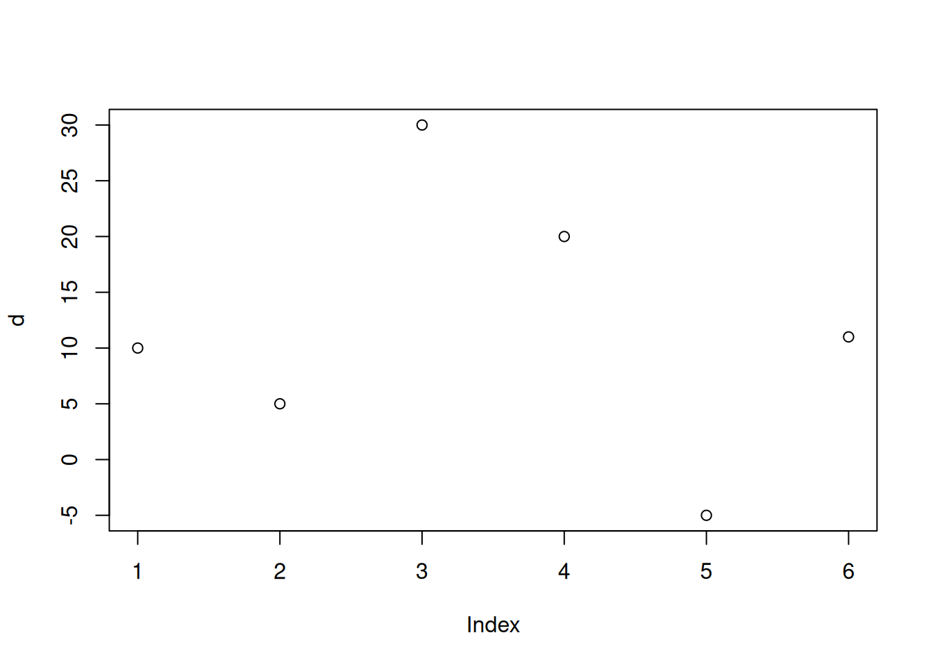
R automatically labels the axis according to what is shown - and the name of the object (here d). There are several options to enhance the plot such as setting a title, rename the axis, or adjusting the way the data are shown.
# Create the data vector d <- c(10, 5, 30, 20, -5, 11) plot(d, main = "Figure Title", xlab = "index/position in the vector", ylab = "measurement", type = "l", col = 4, lwd = 3) 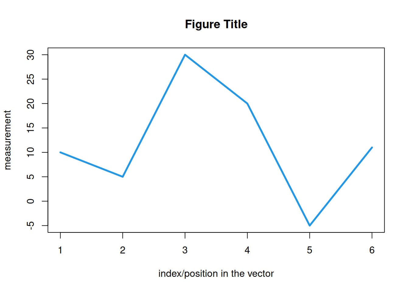
For more details check out the manual page ?plot and/or the Plotting chapter. We can also use it to plot two vectors (same length) against each other. The example below visualizes the sine function between \(-\pi\) and \(+\pi\).
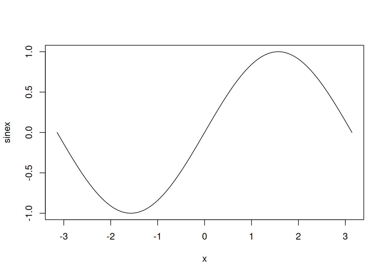
We can also plot functions in R using plot(<function name>). The function is then evaluated along the x-axis. Only works for functions taking up one value x as first input argument. By default, the function is evaluated between 0 and 1, however, we can specify this using custom x-limits.
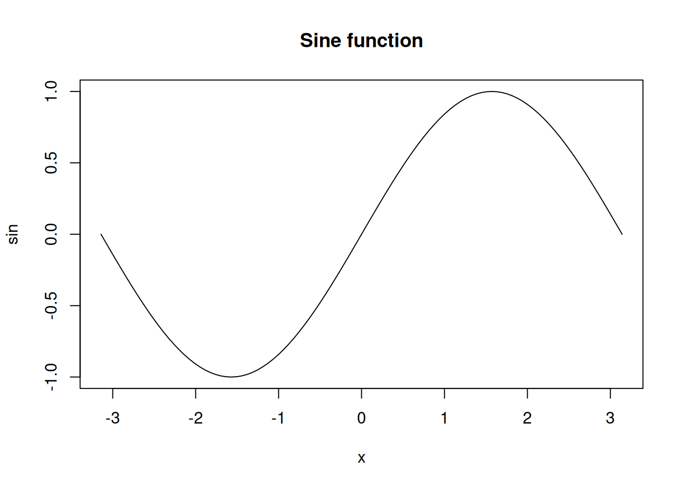
Other functions might be cos(), sqrt(), log(), … Feel free to try it yourself!
Bar plot
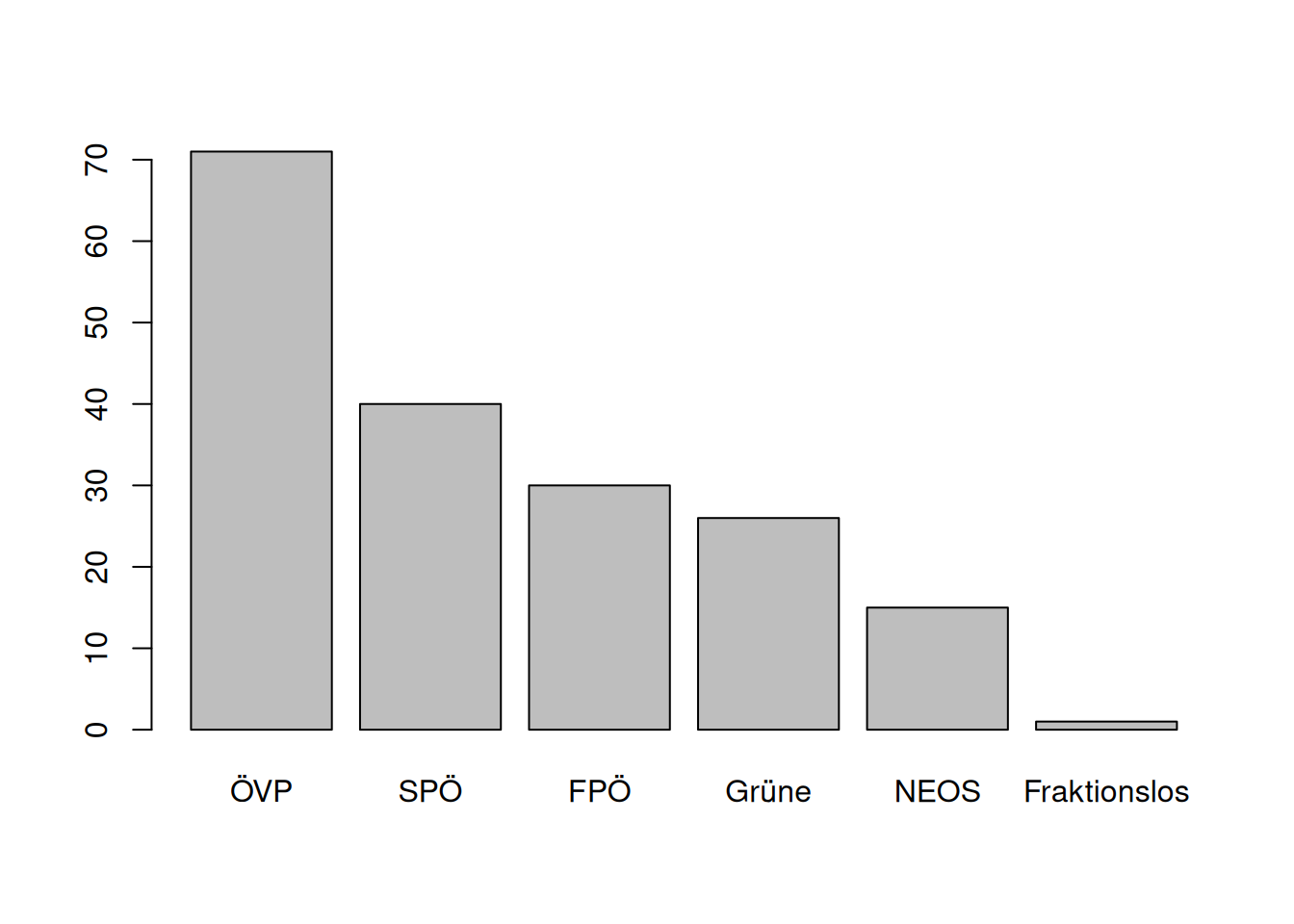
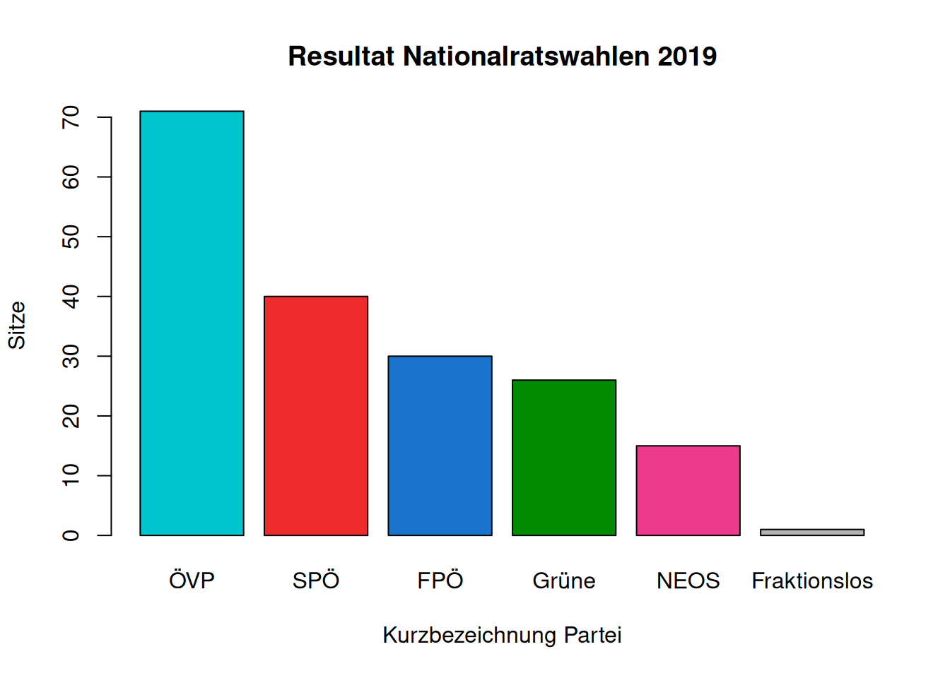
Bar plots are typically used to visualize data for specific groups or classes. Let us assume we would like to visualize the outcome of the latest Austrian legislative election from 2019 (Nationalratswahlen; source wikipedia) and plot the number of seats the parties got out of the election.
This is a classical example to use a named vector in combination with barplot().
Again, we can modify the look and feel to our wishes:
Pie plot
An alternative plot type are pie plots. Keep in mind that pie plots are often not the most effective way of visualizing data. However, if needed, we can do it as follows:
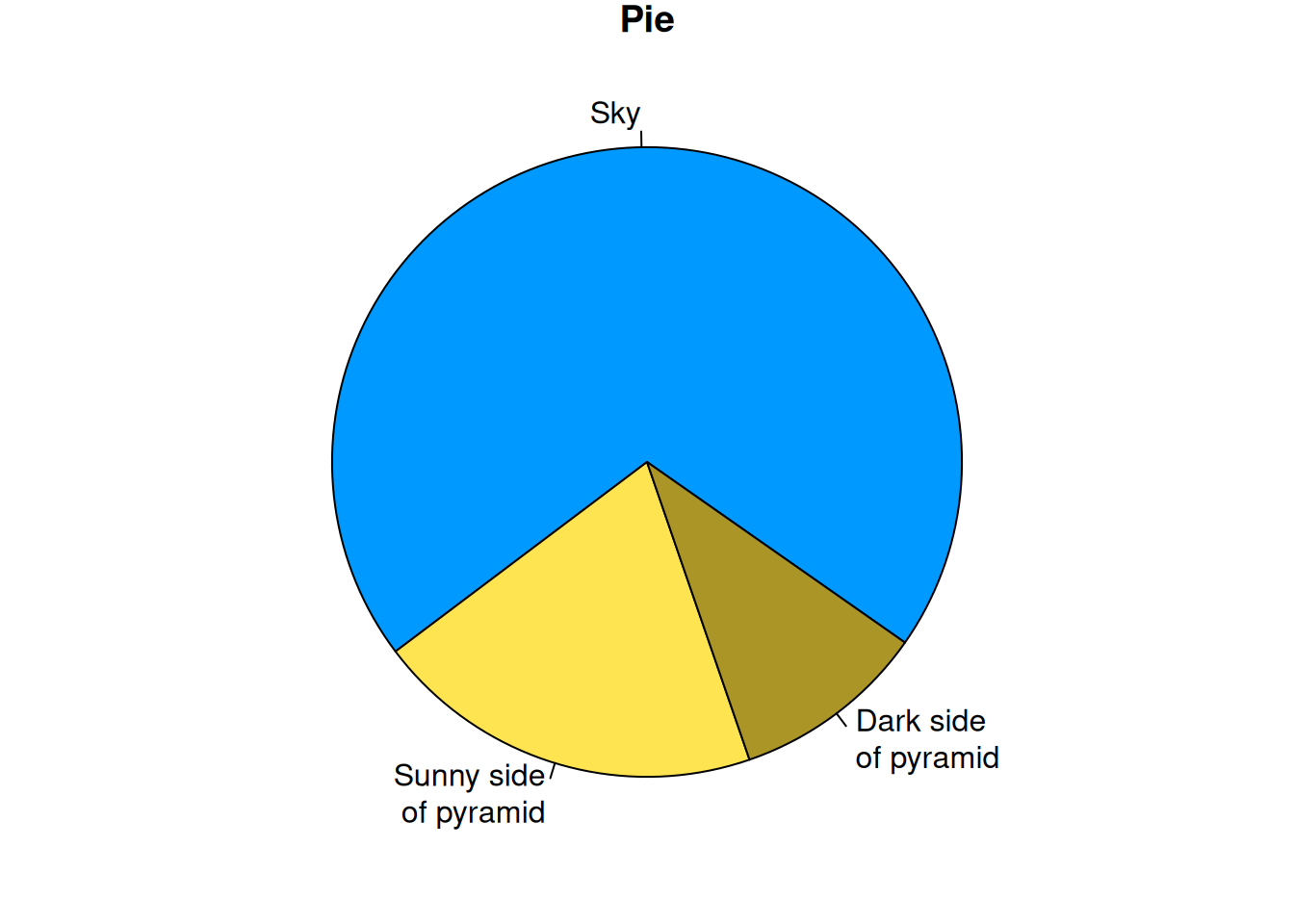
Again, if we have a named vector, R automatically takes the names to label the different sections of the pie (see ?pie for more customization options).
Histograms
A way to visualize large amounts of numeric values are histograms. Histograms show the distribution of the data. For demonstration, let us draw 1000 random values from a standard normal distribution (rnorm(1000)).
We can now see how they are distributed (should show a normal distribution centered around 0 with a variance/standard deviation of 1):
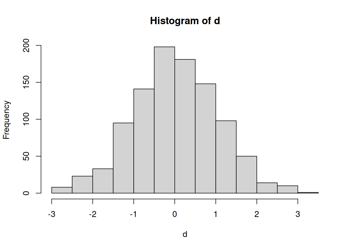
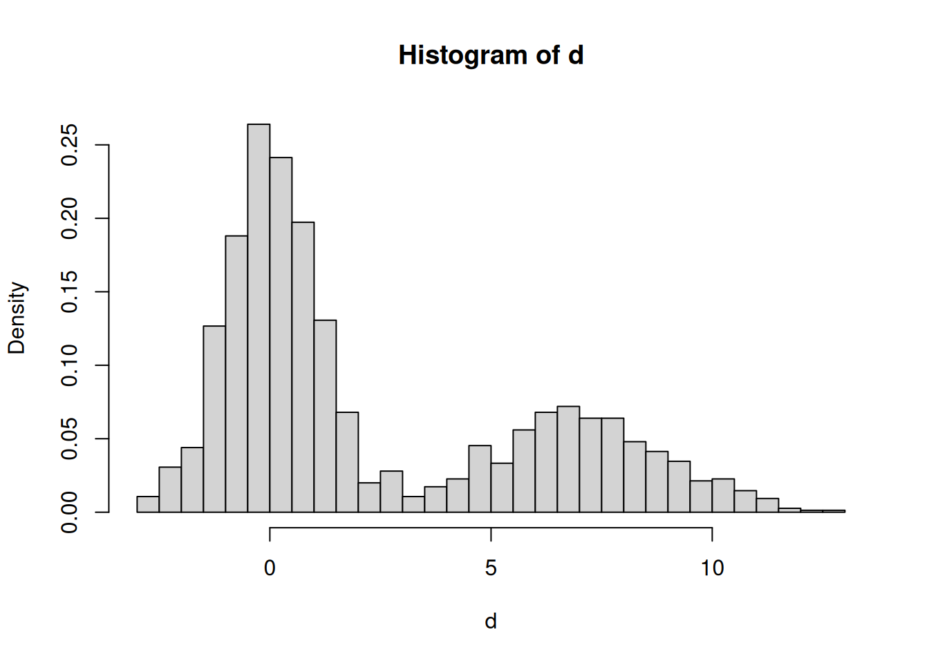
Another example: Mixing random values by drawing 1000 out of the standard normal distribution (with mean 0 and standard deviation 1) and 500 from a normal distribution with mean 7 and standard deviation 2:
Box-and-Whisker plot
An alternative way to show the distribution of numeric values are Box-and-Whisker plots.
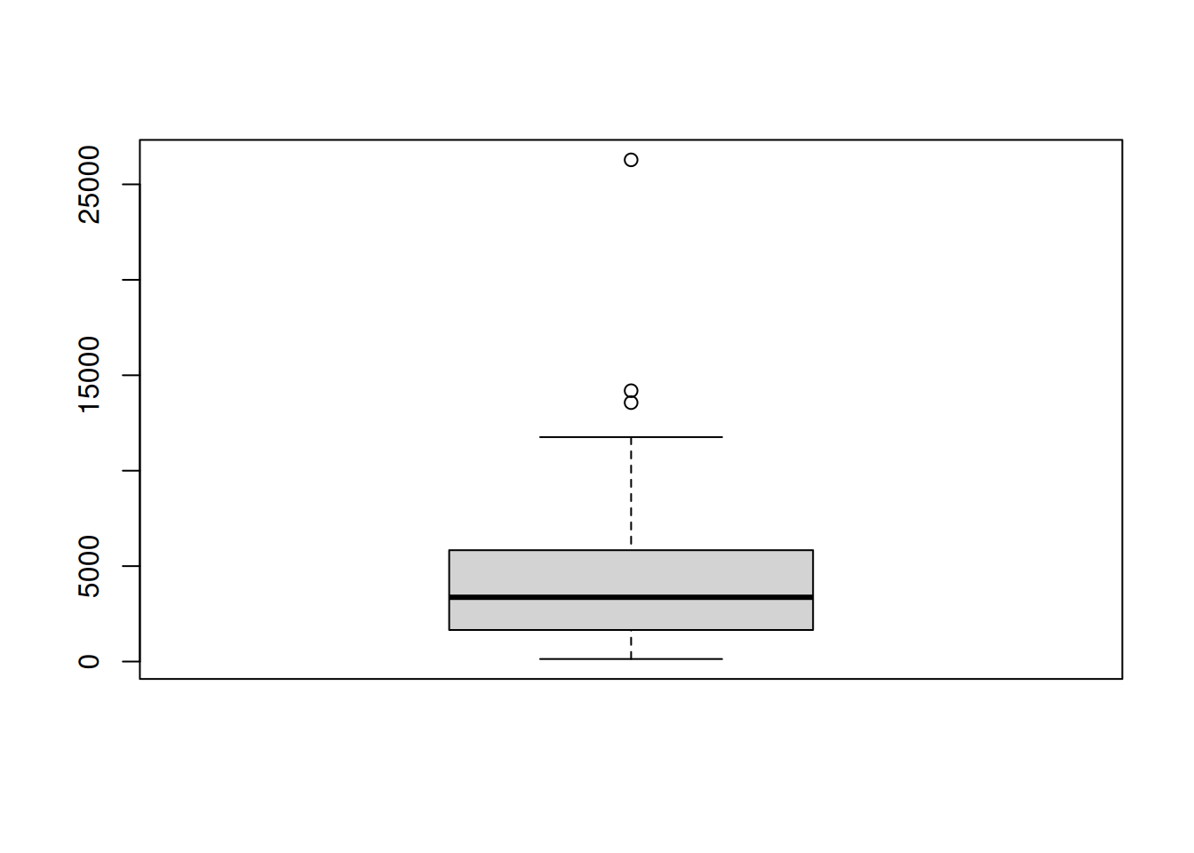
## Min. 1st Qu. Median Mean 3rd Qu. Max. ## 132.5 1668.0 3366.4 4240.6 5753.1 26284.2 The box (gray box) shows the 1th, 2nd (median) and 3th quartile, the same as returned by summary(). The Whiskers (lines) show the data which lie within 1.5 times the inner quartile range from the box, while outliers (those being further away) are plotted as dots. The full range of the plot also shows the minimum/maximum of the data.
Box-and-Whisker plots are especially useful to compare data from different groups, something shown at a later time.
How To Create A Vector In R Studio
Source: https://discdown.org/rprogramming/vectors.html
Posted by: linseymarban.blogspot.com

0 Response to "How To Create A Vector In R Studio"
Post a Comment